Training algorithm

The reinforcement learning algorithm described hereinafter is implemented in learn.py (Learn).

Introduction

The optimal value function is approximated by \(\hat{v}(s; {\bf w}^*)\), a function computed by a multi-layer neural network with weight vector \({\bf w}\).

The Bellman optimality equation for the approximate value function is

\[\begin{equation} \hat{v}(s; {\bf w}^*) = \min_a \sum_{s'} \text{Pr}(s'|s,a) [ 1 + \hat{v}(s'; {\bf w}^*)] \qquad \forall s \neq s^\Omega \end{equation}\]

with \(\hat{v}(s^\Omega; {\bf w}^*) = 0\).

The problem consists in finding the weights \({\bf w}^*\) that allow this equation to be satisfied “at best”, that is, the weights that minimize the residual error. This residual error, called the Bellman optimality error, reads

\[\begin{equation} L({\bf w}) = \mathbb{E}_{s} \left[ \min_a \sum_{s'} \text{Pr}(s'|s,a) [1 + \hat{v}(s'; {\bf w})] - \hat{v}(s; {\bf w}) \right]^2 \end{equation}\]

where the expectation is taken over belief states \(s\) visited when following the policy \(\hat{\pi}\) derived from \(\hat{v}\) and defined by

\[\begin{equation} \hat{\pi}(s; {\bf w}) = \text{argmin}_a \, \sum_{s'} \Pr(s'|s,a) [1 + \hat{v}(s'; {\bf w})]. \end{equation}\]

The functional \(L({\bf w})\) is known as the “loss function”, and “training” the network then refers to the iterative update (through stochastic gradient descent) of the weights \({\bf w}\) so as to minimize this loss function.

Deep neural network

Preprocessing

The belief state, which contains both the agent’s position (an \(n\)-tuple) and the source probability distribution (an \(N^n\) array, with \(N\) the linear grid size and \(n\) its dimensionality), is equivalently represented as a source probability distribution centered on the agent (a \((2N-1)^n\) array). This transformation, illustrated below, is applied to the belief state before using it as an input to the neural network.

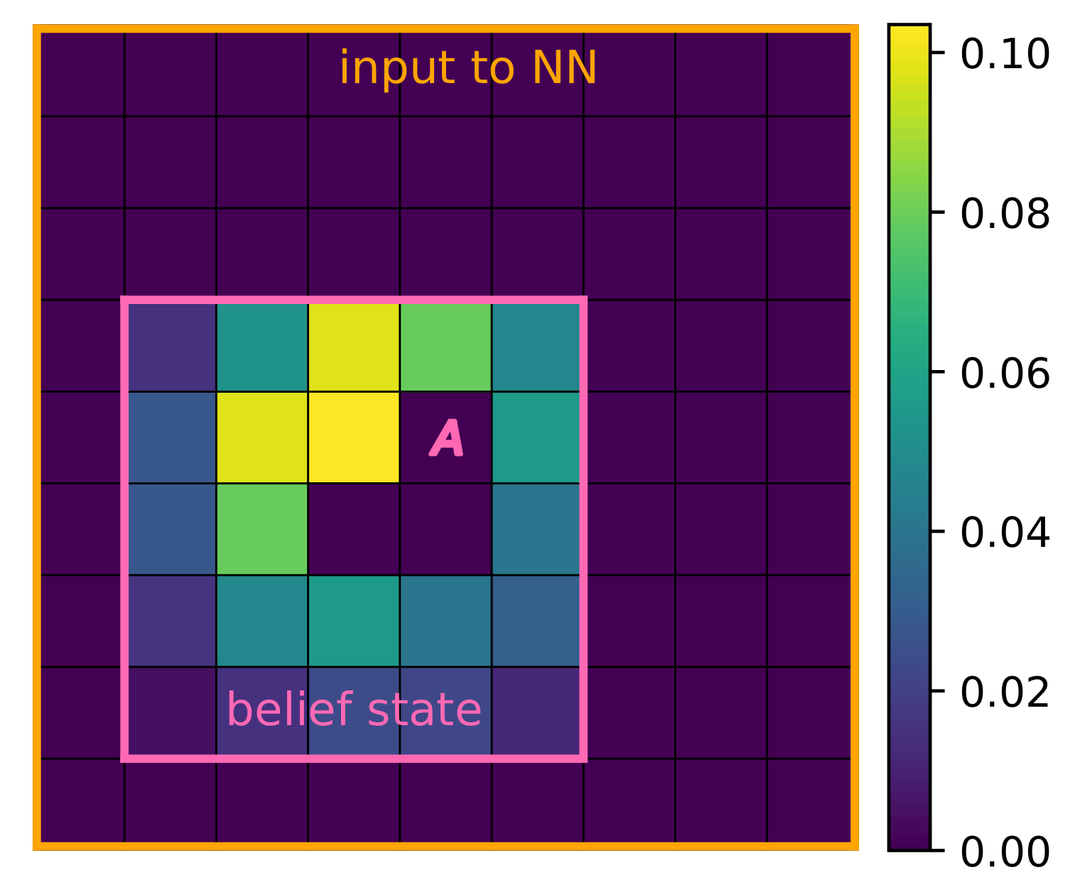
The belief state (pink border and agent) is transformed into a probability distribution centered on the agent (orange border).

Architecture

The neural network consists of fully connected layers: the input layer, followed by hidden layers with rectifier linear units (ReLU) activations, and a linear output layer. The network size (number of hidden layers and number of neurons per hidden layer) can be chosen by the user with the FC_LAYERS and FC_UNITS parameters.

Near-optimal policies can be obtained if large enough neural networks are used. Typically 3 hidden layers are sufficient for most cases, and an increasing number of neurons per layer is required for increasing problem sizes.

Algorithm

The training algorithm is a custom model-based version of DQN (Mnih et al., Nature, 2015). The pseudo-code is given below.

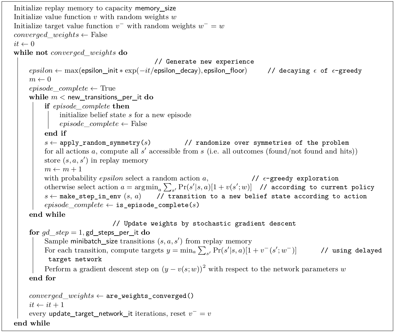
Pseudo-code for the training algorithm (based on DQN).