Description
The source-tracking problem is a POMDP (partially observable Markov decision process) in which the agent seeks to identify the true location of an imperfectly observed stationary target (a source of odor). The environment is an \(n\)-dimensional Cartesian grid and the source, invisible to the agent, is located in one of the cells. At each step, the agent moves to a neighbor cell and receives an observation (odor detection), which provides some information on how far the source is. The agent has a perfect memory and a perfect knowledge of the process that generates observations. How should the agent behave in order to reach the source in the smallest possible number of steps?
We denote \({\bf x}^s\) and \({\bf x}^a\) the source and the agent locations (\(n\)-tuples of integers), respectively. Allowed actions are moves to a neighbor cell along the grid axes, for example in 3D the set of allowed actions is {‘north’, ‘south’, ‘east’, ‘west’, ‘top’, ‘bottom’}, and staying in the same location is not allowed. After moving to a cell, either the source is found (event \(F\)) and the search is over, or the source is not found (complementary event \(\bar{F}\)) and the agent receives a stochastic sensor measurement \(h\) (“hits”), which represents the integer number of odor particles detected by the agent. Hits are received with conditional probability \(\text{Pr}(h | {\bf x}^a,{\bf x}^s)\) specified by an observation model. We encompass the presence/absence of the source and the number of hits in a single observation variable \(o\). Possible observations are \(o \in \{ F, (\bar{F}, 0) , (\bar{F}, 1), (\bar{F}, 2), \dots \}\).
We denote \(p({\bf x})\) the discrete probability distribution of the source being in each grid cell, that is \(p({\bf x}) = \text{Pr}({\bf x}^s = {\bf x})\). After each action and observation, \(p({\bf x})\) can be updated using Bayesian inference. The agent has access to its position \({\bf x}^a\) and to the distribution \(p({\bf x})\). In the POMDP terminology, this defines a belief state \(s=[{\bf x}^a, p({\bf x})]\), as illustrated below. Finding the source is a special belief state \(s^\Omega\) where the source position is known and matches the agent position: \(s^\Omega=[{\bf x}^a, \delta({\bf x} - {\bf x}^a)]\). The agent’s behavior is described by a policy, denoted \(\pi\), which maps each belief state to an action.
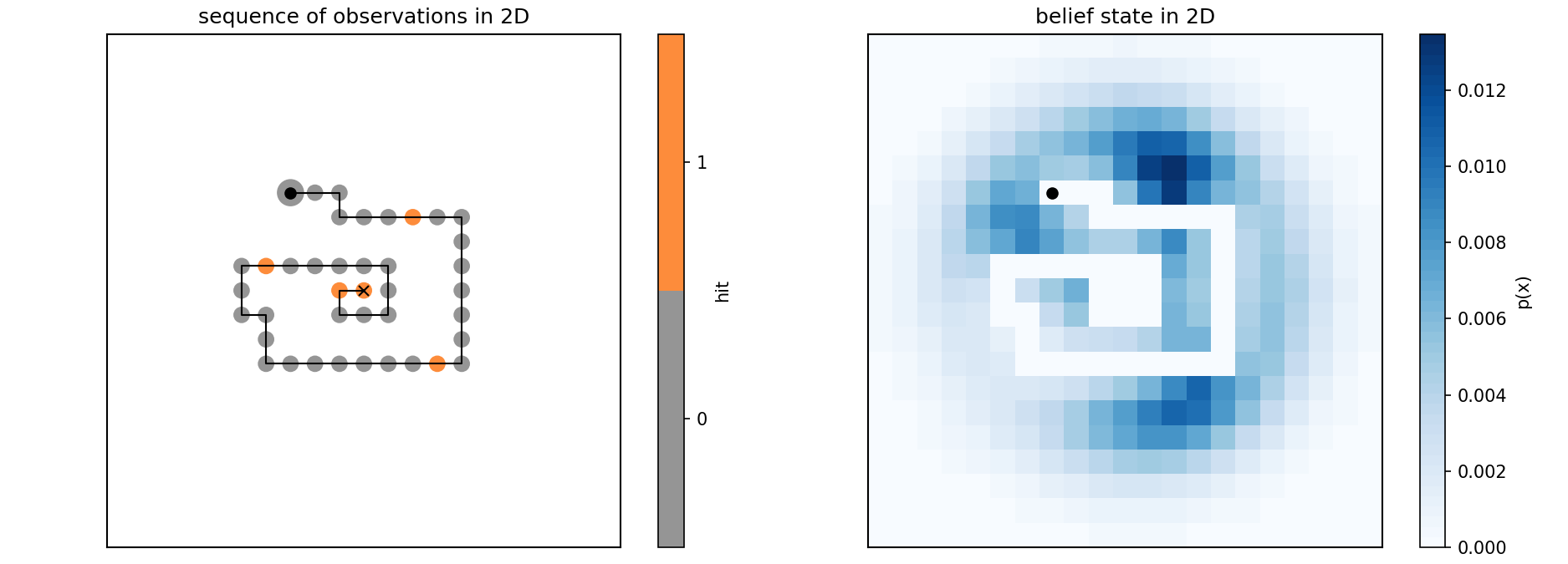
Example of an observation sequence and corresponding belief state.
The search proceeds as follows:
Initially
The belief state is \(s_0=[{\bf x}^a_0, p_0({\bf x})]\), where the agent location \({\bf x}^a_0\) is at the center of the domain and where the prior distribution of source location \(p_0({\bf x})\) is drawn randomly from the set of prior belief states.
The source location \({\bf x}^s\) is drawn randomly according to \(p_0({\bf x})\).
At the \(t^\text{th}\) step of the search
Knowing the current belief state \(s_t=[{\bf x}^a_t, p_t({\bf x})]\), the agent chooses an action according to some policy \(\pi\): \(a_{t} = \pi(s_t)\).
The agent moves deterministically to the neighbor cell associated to \(a_{t}\). This move is associated to a unit cost. The agent’s position is updated to \({\bf x}^a_{t+1}\).
The agent receives an observation \(o_{t}\) and the source location distribution is updated using Bayes’ rule to \(p_{t+1}({\bf x})\).
If \(s_{t+1} = s^\Omega\), that is \({\bf x}^a_{t+1} = {\bf x}^s\), the search terminates and the agent receives no more costs.
Otherwise, the search continues to step \(t+1\).
Each episode (each search) is a sequence like this:
and the cumulated cost of an episode is equal to the number of steps \(T\) to termination (which can be infinite if the source is never found).
Episodes can be visualized with visualize.py (Visualize).
A step-by-step illustration depicting how a search proceeds is provided.
Some examples of episodes are shown in the gallery.
With our initialization protocol, the source-tracking POMDP is parameterized by only three dimensionless parameters:
the dimensionality \(n\), called
N_DIMSin the codethe dimensionless problem size \(L\), called
LAMBDA_OVER_DXin the codethe dimensionless source intensity \(I\), called
R_DTin the code